Following my article on Software Engineering Daily, here are some practical things that will help you if you’re considering taking on a technical book project.
Identifying a Publisher
While it is easy to self-publish today. The recognition comes from having worked with a traditional publisher as they have processes that ensure a level of quality. Not all publishers are equal, and some publishers are attributed with more prestige than others. In addition to this, some publishers are willing to take a risk on a subject and/or author. Have a look at the titles already published, and whether there are any publishers you can connect to.
When comes to contacting the publishers, most of their websites will have a page for recruiting authors. Some are easier to find than others. Here are a couple:
If, or when you get to talk to a publisher it is worth ensuring you understand how their editorial process works and what is expected from you? Plus what happens if you find yourself in the position of not being able to work to the original schedule. Day-to-day work can get in the way which you hadn’t expected.
For a long time, I’ve tracked and read articles on Software Engineering Daily. We’ll day represents what is hopefully the first of many articles that we will write for them. The article is about the kind of people that make technical book authors, and the perception we have of authors – so if you’re interested check it out here.
The 12 Factor App definition is now ten years old. In the world of software that is a long time. So perhaps it’s time to revisit and review what it says. As I have spent a lot of time around Logging – I’ve focussed on Factor 11 – Logging.
I have been fortunate enough to present at the hybrid JAX London conference on this subject. It was great to get out and see people at a conference rather than just with a screen and a chat console of online-only events.
Having previously blogged about being a fan of Railroad diagrams (here) as a means to communicate language syntax, I have been asked about some of the ways details should be represented. I’ve looked around and not actually found an easy-to-read for ‘newbies’ guide to reading railroad diagrams. A lot of content either focuses on the generator tools or how the representation compares to BNF (Backus Naur Form) – all very distracting. So, I thought as an advocate, I should help address the gap (the documentation with TabAkins tool does a good job of explaining things, but its focus is on the features provided rather than understanding the notation).
Reading Railroad Diagrams
The following table provides all the information to help you interpret the Railroad Diagrams, and create syntax representations.
If you’re only interested in understanding the notation, read just the first two columns.
If you want to see examples of how to create the diagram, then the 3rd column will help.
Note: Clicking on the diagrams will result in a bigger version of the image being displayed.
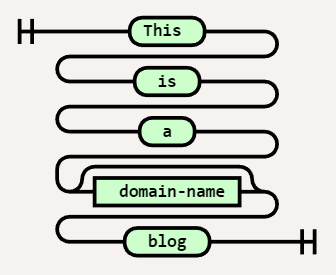
The start and end of an expression are shown with vertical bars. The expression is read from left to right following a path defined by the line(s).
Diagram(
Terminal('This '),
Terminal(' is '),
Terminal(' a '),
Terminal(' mp3monster '),
Terminal(' blog ')
)
Larger diagrams may need to be read both across and down the page to make it sensibly fit a page like this.
Diagram( Stack(
Terminal('This '),
Terminal(' is '),
Terminal(' a '),
Terminal(' mp3monster '),
Terminal(' blog '))
)
We can differentiate between literal values and ‘variables’ by shape. A square shape should denote a variable, and a lozenge represents a literal. I have to admit to sometimes getting these the wrong way around, but as long as the notation is used consistently in an expression, it isn’t too critical. In this example, we have replaced mp3monster with the name of a variable called domain-name. So if I set the variable domain-name = mp3monster then I’d read the same result.
Diagram( Stack(
Terminal('This '),
Terminal(' is '),
Terminal(' a '),
NonTerminal(' domain-name'),
Terminal(' blog '))
)
We can make parts of an expression optional. This can be seen by following an alternate path around the optional element. In this case, we’ve made the domain-name optional. Assuming domain-name = mp3monster, we could get either: – This is a mp3monster blog OR – This is a blog
Diagram( Stack(
Terminal('This '),
Terminal(' is '),
Terminal(' a '),
Optional(
NonTerminal(' domain-name')), Terminal(' blog ')) )
We can represent optionality by having the flow split to multiple values. Those values could be either literal values or variables. In this case, we now have several possible names in the blog with the choices being mp3monster, phil-wilkins, cloud-native, or the contents of the variable domain-name. So the expression here could resolve to (assuming domain-name = something-else): – This is a mp3monster blog OR – This is a phil-wilkins blog OR – This is a cloud-native blog OR – This is a something-else blog It is typical for the option most likely to be selected to be the value that is directly in line with the choice. Here that would mean the default would be phil-wilkins
Diagram( Stack(
Terminal('This '),
Terminal(' is '),
Terminal(' a '),
Choice(1,
' mp3monster', ' phil-wilkins ', ' cloud-native ', NonTerminal('domain-name')), Terminal(' blog ')) )
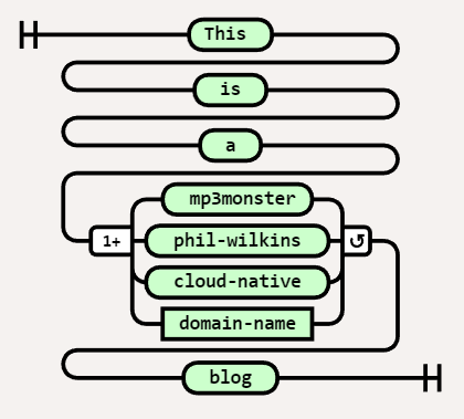
We can have variations on a choice where we can express the choice as being any of the options (one or more e.g. mp3monster and cloud-native) or all of the choices. These scenarios are differentiated by the additional symbols before and after the choice.
Diagram( Stack(
Terminal('This '),
Terminal(' is '),
Terminal(' a '),
MultipleChoice(1,
'any',' mp3monster', ' phil-wilkins ', ' cloud-native ', NonTerminal('domain-name')), Terminal(' blog ')) )
We can represent the looping with the inclusion of an additional literal(s) or variable(s) by having a second line from the right (exit) of a literal or variable and flowing back into the left (entry) of a literal or variable. Then in the loop of the flow below are the variable(s) or literal(s) that go around between each occurrence of the loop. If our variable was a list now i.e. domain-name = [‘ mp3monster’, ‘cloud-native’] then this would resolve to : This is a mp3monster and cloud-native blog
Diagram( Stack(
Terminal('This '),
Terminal(' is '),
Terminal(' a '),
OneOrMore(
NonTerminal('domain-name'), [' and '])), Terminal(' blog ') )
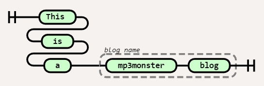
We can group literals and variables together with a label. These groupings are denoted with a dashed line and usually include some sort of label. In our example, we’ve grouped two literal values together and called that group the blog name.
Diagram( Stack(
Terminal('This '),
Terminal(' is '),
Terminal(' a '),),
Group(Sequence(
Terminal(' mp3monster '), Terminal(' blog ')), ['blog name']) )
All of these constructs can be combined so you can do things like making choices optional, and iterate over multiple variables and literals.
Sometimes the number of options in a choice can get impractically large to show in a Railroad diagram. One way to overcome this is to show the first and last options and an ellipsis. We can then wrap it with a comment that directs the reader to the complete list of choices. This way the diagram continues to be readable – the most valuable part of the diagram and easy to locate the specific fine details.
Diagram( Stack( Terminal(‘This ‘), Terminal(‘ is ‘), Terminal(‘ a ‘), Group(Choice(1, ‘ mp3monster’, ‘ … ‘, ‘ cloud-native ‘), [‘ See Section X for full list’]), Terminal(‘ blog ‘)) )
I was fortunate enough to be invited to join LogRocket‘s Podcast (PodRocket) to discuss some of the insights and considerations relating to API Streaming that I presented at a reference conference. To hear more go checkout :
If you’d like to see more from the presentation, go here.
When it comes to CI/CD deployments, something that doesn’t show very often in documentation is the pros and cons of running your worker nodes as containers in a Kubernetes environment or as (virtual) machines in a cloud environment.
We’ve all encountered decision trees at one time or another as a means to determine an answer based on a set of inputs. The problem with decision trees is that they are binary in nature. The answer is always yes or no.
But life is not binary. This is often best underlined by the classic joke of asking an architect what the right thing to do is, and you’ll get the answer ‘it depends‘. The art of being an architect is working out what the right trade-offs are when coming to a decision. This is fine, but to know all the factors (or trade-offs) that need to be considered requires a wealth of experience (a rare and expensive asset) or someone capturing these insights in a consumable manner that enables people who will understand how to use imparted wisdom, rather than try to blindly follow binary decisions.
This is where decision Matrices, or as I was introduced to them ‘Stress Tests’ – so called because the matrix is made up of a factor or ‘stressor’ are tested against one or more options. Each slot in the matrix can either be marked as yes/no or scored on the range (for example 1-5) on alignment to meeting the stressor. If you’re doing a product selection then the options are the different products. But equally the options could be an architectural pattern.
This is probably best illustrated. So the following Matrix looks at different programming languages against a range of different stressors. This isn’t a realistic case, but sufficient to help convey the idea. (The assessments in this matrix are not comprehensively researched, so feel free to argue)
Java
Python
Ruby
C++
Single binary for multiple OS and architectures
5
5
4 1
1
Language evolves quickly to provide standardized libraries for common needs
5
5
4
3
Suitable for scripting and application development
42
5
4
1
Readily available skills
4
5
33
33
Ruby has several variants such as JRuby, Ruby with a C core – this has the potential to impact
Use of Shebang or overlaying with Groovy makes Java more usable as a scripting language
Not so commonly taught in educational settings which typically favor Python and Java
As you can see to help use the matrix we can add elaboration notes. To use the matrix we simply determine which stressors are most important or not and then score the different options. So if I wanted to use the matrix to determine which language is most suitable for developing a deployment utility then we know from the use case performance is less critical, portability is important, and skills should outweigh language evolution. Based on that the answer should resolve to Python failing that Java would be good enough.
While our question and its outcome is fairly obvious, in more nuanced situations the stress test gives several benefits:
The decision process becomes transparent and easily communicated.
The hard work is in developing the stressors and researching the different options in terms of how they fit with stressors.
The matrix can be re-used, to help achieve other decisions. What if I was looking at the most suited solution for running data analytics that can maximize GPUs?
Through the use of the stress test we can translate the ‘it depends‘ to a more concrete but rationalized decision.
My blogging activities have expanded a little bit further. Oracle staff (particularly those involved with Product Management) and the Ace community have been contributing to a Medium publication called Oracle Devs (go here). The content here is 1st rate, technically comprehensive, and from some exceptional technical people. So I’d recommend tracking it if you aren’t already and I feel very honored to have several posts already included, which can be found at:
Those that follow me here, not o worry, this is the center of the universe for my blogging activity, and I will tie back anything that is unique to Medium o posts here.
In addition to that, I do also have a profile on the official Oracle Blog (here), and a range of posts have also been picked up via the PaaSCommuniy which haven’t been directly linked to my Oracle blog profile but can be found with this link
One of the areas I present publicly is the use of Fluentd. including the use of distributed and multiple nodes. As many events have been virtual it has been easy to demo everything from my desktop – everything is set up so I can demo things very easily. While doing this all on one machine does point to how compact and efficient Fluentd is as I can run multiple instances concurrently it does undermine distributed capabilities somewhat.
Add to that I now work for Oracle it makes sense to use OCI resources. With that, I have been developing the scripts to configure Ubuntu VMs to set up the demo environments installing Ruby, Fluentd, and various gems needed and pulling the relevant configurations in. All the assets can be found in the GitHub repository https://github.com/mp3monster/logging-demos. The repository readme includes plenty of information as well.
While I’ve been putting this together using OCI, the fact that everything is based on Ubuntu should mean it can be run locally on VMs, WSL2, and adaptable for MacOS as well. The environment has been configured means you can still run on Ubuntu with a single node if desired.
Additional Log Destinations
As the demo will typically be run on OCI we can not only run the demo with a multinode setup, we have extended the setup with several inclusion files so we can utilize OCI services OpenSearch and OCI Log Analytics. If you don’t want to use these services simply replace the contents of several inclusion files including files with the contents of the dummy_inclusion.conf file provided.
Representation of the Demo setup
The configuration works by each destination having one or two inclusion files. The files with the postfix of label-inclusion.conf contains the configuration to direct traffic to the respective service with a configuration that will push log events at a very high frequency to the destination. The second inclusion file injects the duplication of log events to each service. The inclusion declarations in the main node Fluentd config file references an environment variable that should provide the path to the inclusion file to use. As a result, by changing the environment variable to point to a dummy file it becomes possible o configure out the use of one of the services. The two inclusions mean we can keep the store declarations compact and show multiple labels being used. With the OpenSearch setup, we have a variant of the inclusion file model where the route inclusion can reference the logic that we would use in the label directly within the sore declaration.
The best way to see the use of the inclusions is to experiment with setting the different environment variables to reference the different files and then using the Fluentd dry-run feature (more on this in the book).
Setup script
The setup script performs a number of tasks including:
Pulling from Git all the resources needed in terms of configuration files and folders
Retrieving the necessary plugins against the possibility of their use.
Setting up the various environment variables for:
Slack token
environment variables to reference inclusion files
shortcut environment variables and aliases
network (IP) address for external services such as OpenSearch
Setting up a folder for OCI tokens needed.
Setting up temp folders to be used by OCI Plugins as a file-based cache.
Feeding the log analytics service is a more complex process to set up as the feeds need to have metadata about the events being ingested. The downside is the configuration effort is greater, but the payback is that it becomes easier to extract meaningful information quickly because the service has a greater understanding of the content. For example, attributing the logs to a type of source means the predefined or default log formats are immediately understood, and maximum meaning can be retrieved from the log event.
Going to OCI Log Analytics does cut out the need for the Connections hub, which would allow rules and routing to be defined to different OCI services which functionally can help such as directing log events to PagerDuty.
's Blog")


You must be logged in to post a comment.